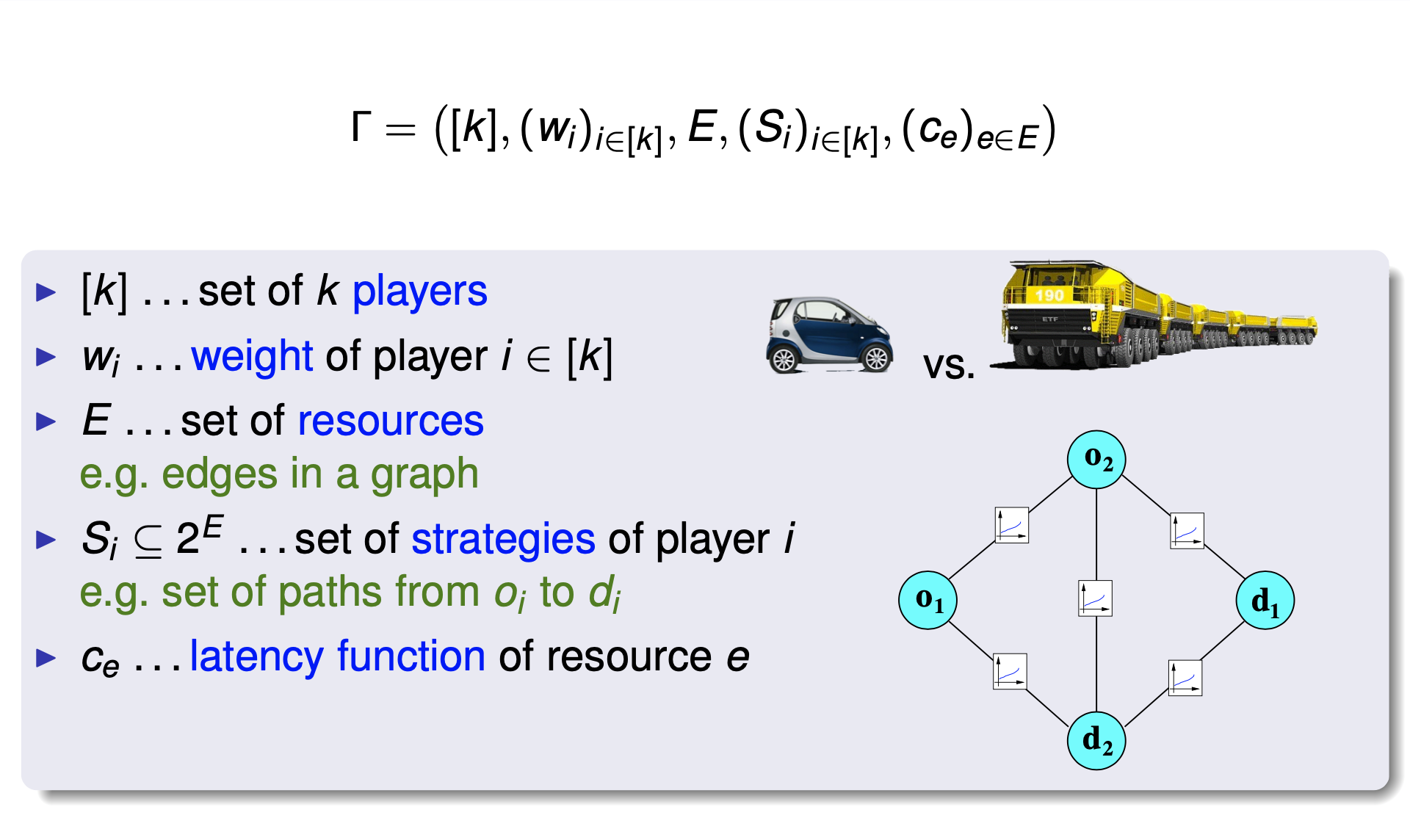
Non-atomic congestion games: Wardrop Model

Wardrop Model

• directed graph G = (V,E)

• kcommodities,oneforeachi∈[k]

  • si , ti … source-sink pair
  • ri … flow demanPd to route from si to ti I normalise: r = i∈[k] ri = 1
  • Pi … set of paths between si and ti

• P = Ui∈[k]Pi a set of paths

• ce : [0,1] → R… latency (cost) function of edge e ∈ E

• continuous, non-decreasing, non-negative

• The triple (G,r,c) is an instance of the routing problem

• Flow and Latency:

  • Flow f: aPflow vector (fP)P∈P
  • f_e= P ∋ e f_P
  • a P flow is feasible if for all i∈[k] P ∈ Pi f_P = r_i

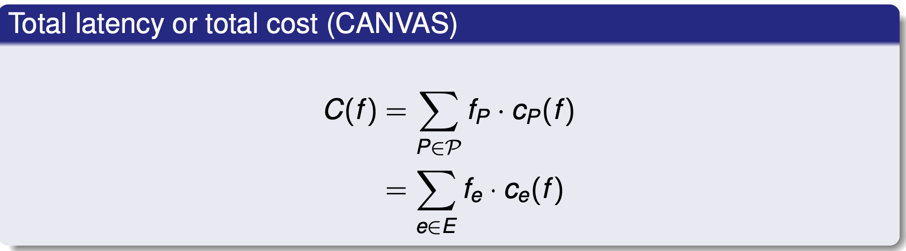
• C_e(f) = c_e(f_e) … edge (lentence / cost)

• C_p(f) = Sum e ∈ P c_e(f) … path latency

• Example:

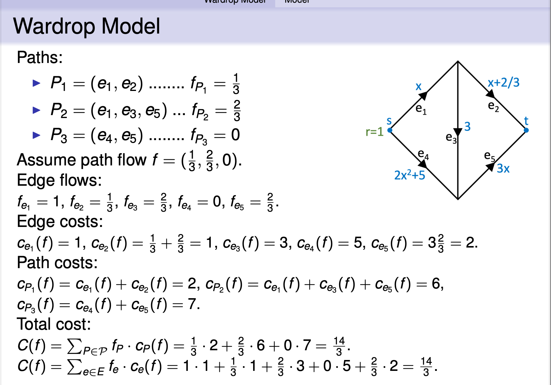
Paths:

• P1=(e1,e2)…fP1 = 1 / 3
• P2 = (e1,e3,e5) … fP2 = 2 / 3
• P3=(e4,e5)…fP3 =0

Assume path flow f = (1/3, 2/3,0).

Edge flows:

fe1 =1,fe2 = 1/3,fe3 = 2/3,fe4 =0,fe5 = 2/3.

Edge costs:

ce1(f)=1, ce2(f)=1/3 + 2/3 =1, ce3(f)=3, ce4(f)=5, ce5(f)=3 * (2/3) =2.

Path costs: cP1 (f ) = ce1 (f ) + ce2 (f ) = 2, cP2 (f ) = ce1 (f ) + ce3 (f ) + ce5 (f ) = 6, cP3 (f ) = ce4 (f ) + ce5 (f ) = 7.

Total cost:

C(f) = Sum fp * cp = 1/3 * 2 + 2/3 * 6 + 0 * 7 = 14/3

C(f)= fe·ce(f)= 1·1 + 1/3 * 1 + 2/3 * 3 + 0 * 5 + 2/3 * 2 = 14/3

• So far,we basically just introduced a flow model.

• In the Wardrop model we assume:

  • flow is controlled by an infinite number of agents

  • each agent is responsible for an infinitesimal fraction of the flow

  • agents strive to minimise their own latency

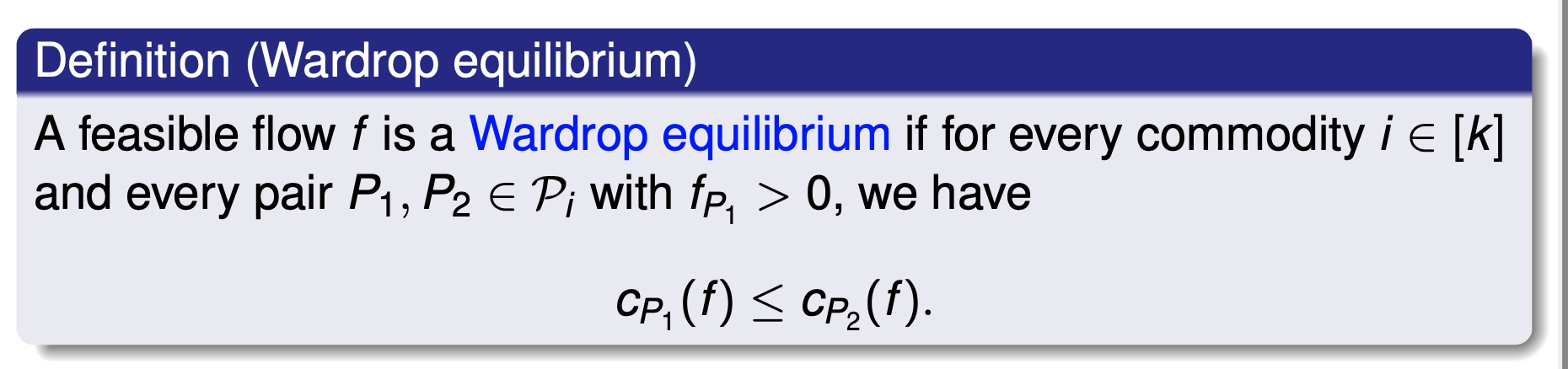
• This implies: All used paths of the same commodity have the same latency.

Optimal Flows & Wardrop Equilibria

• Suppose we are shifting flow from path P1 to P2.

• ⇒ Contribution of edges on P1 to total latency decreases, contribution of P2 increases.

• If decrease on P1 is more than the increase on P2 then total latency decreases.

• ⇒the flow was not optimal.

• Marginal Cost (边际成本)

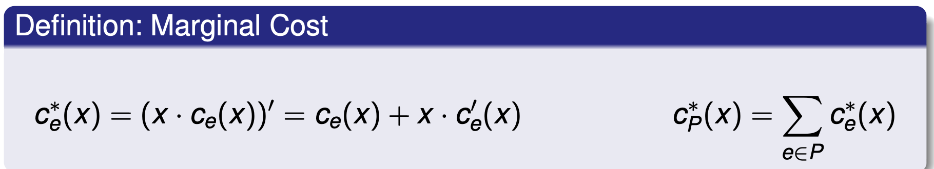
Optimum Flow via marginal costs

Assume x · ce (x ) is convex and continuously differentiable for all e ∈ E

• Lemma 3.1 (Characterisation of optimal flows) 最优流的特点

A feasible flow f is optimal if and only if for all commodities i ∈ [k], and paths P1,P2 ∈ Pi with fP1 > 0, we have cP∗ (f) ≤ cP∗ (f).

• Observe the similarity in the characterisation of optimal flows and Wardrop equilibria.

• Theorem 3.2 (Wardrop equilibrium vs. Optimum). 比较

A feasible flow f is optimal for (G,r,c) if and only if f is a Wardrop equilibrium for (G,r,c∗).

• Theorem 3.3 (Existence and essential uniqueness)

(a) Every instance (G,r,c) admits a Wardrop equilibrium. (CANVAS)

(b) If f and ̃f are Wardrop equilibria, then ce(f) = ce( ̃f) for every e ∈ E.

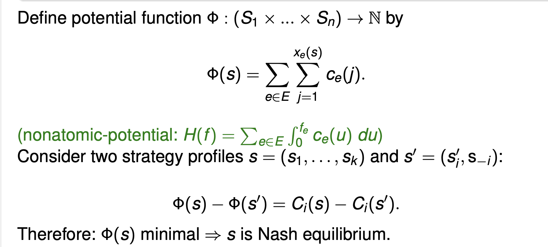
• Proofs are based on the following potential function [ BECKMANN, MCGUIRE, WINSTON,1956] :

  $H(f) = \sum_{e ∈ E} h_e(f_e)$

  $he(x) = \int_0^x ce(u) du$

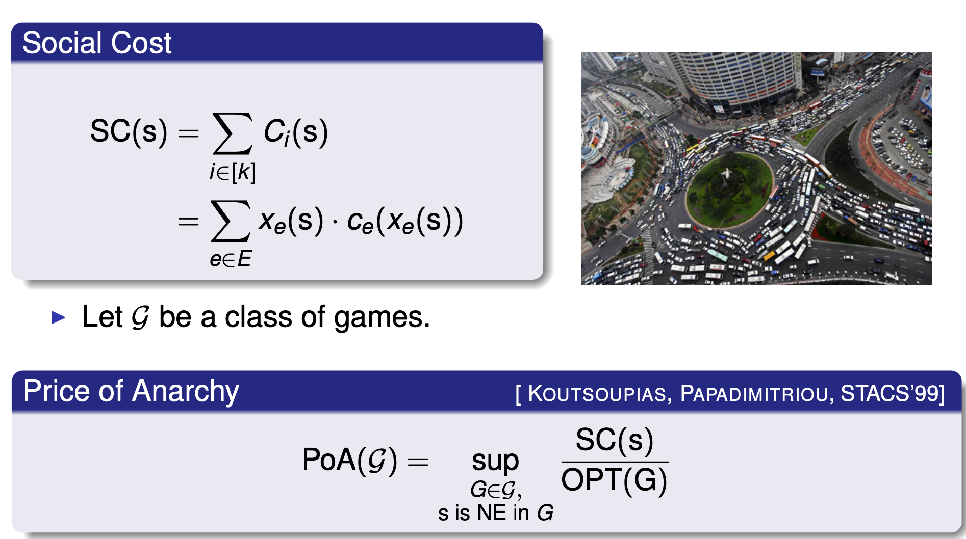
Price of Anarchy

• Let f be a Wardrop equilibrium and f ∗ be an optimum for (G, r , c).

ρ(G,r,c)= C(f) / C(f∗)

• Theorem 3.4 (polynomial latency functions) 多项式延迟函数

Suppose latency functions are of the form $ce(x) = \sum_{i = 0}^d ae&, i * xi$ with nonnegative coefficients, Then ρ(G, r, c) <= d + 1

• Theorem 3.5 (linear latency functions) 线性延迟函数

Suppose latency functions are linear with non-negative slope and offset. Then, ρ(G,r,c) = 4/3.

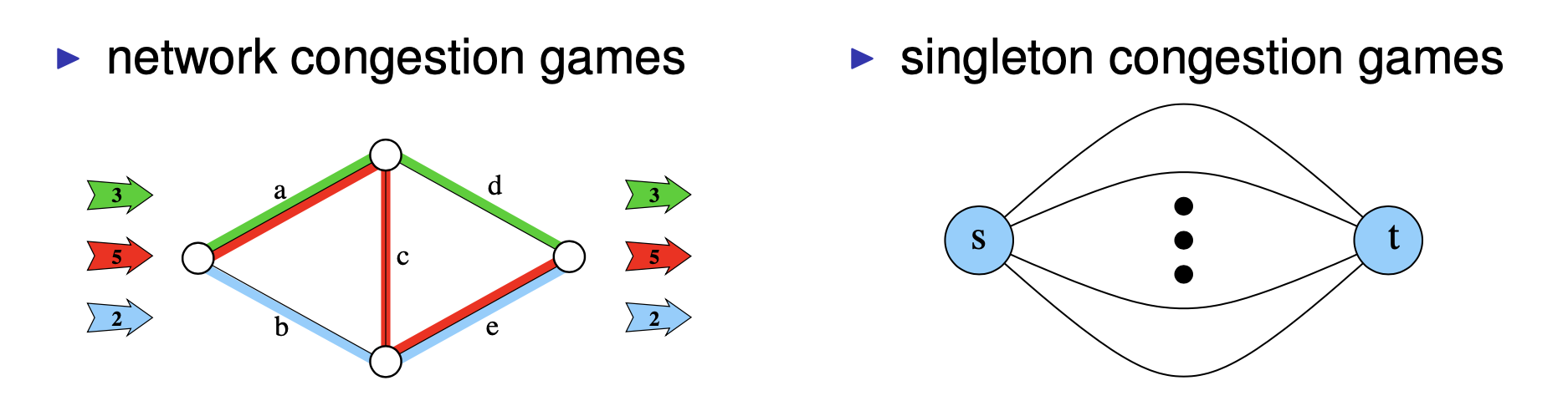
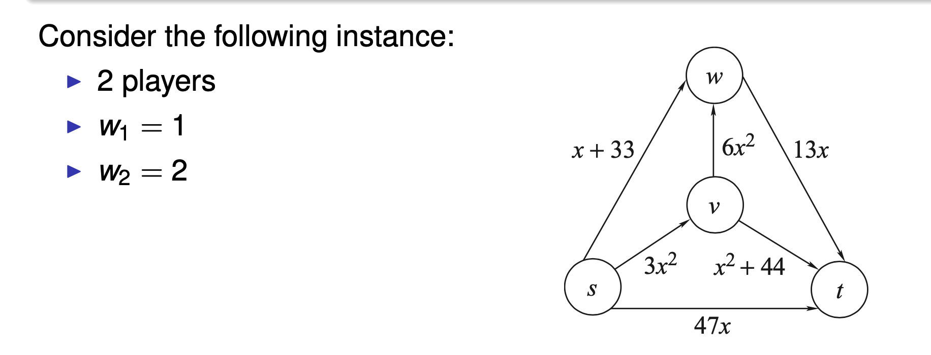
(Atomic) congestion games

• (Weighted) congestion games

  

  • unweighted congestion games(or simply congestion games):

    wi =1 for all players i ∈[k]

  • symmetric games:

    Si = Sj for all player i,j ∈ [k]

  

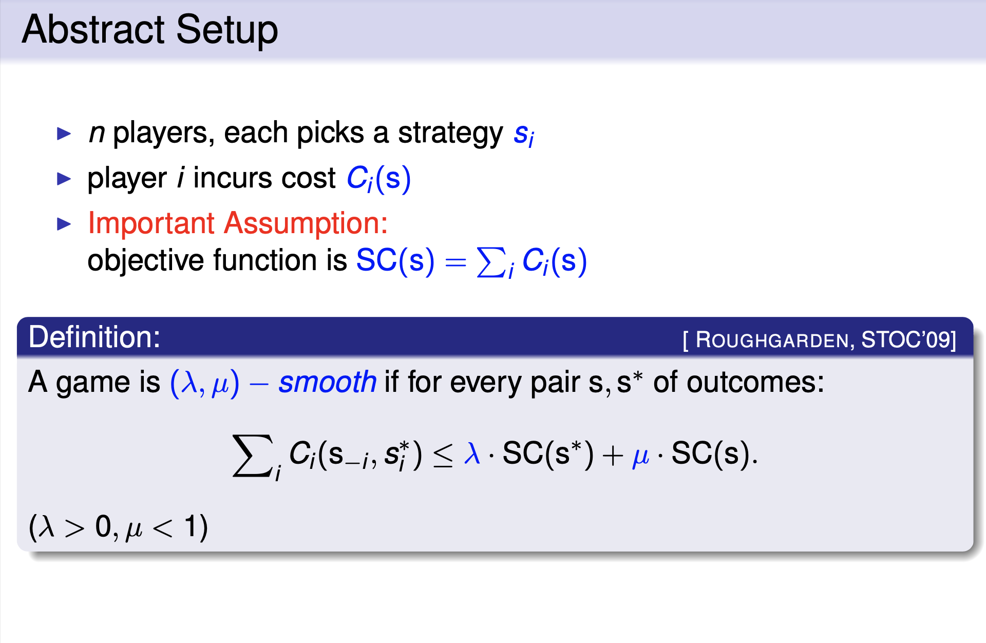
Private Cost and Social Cost

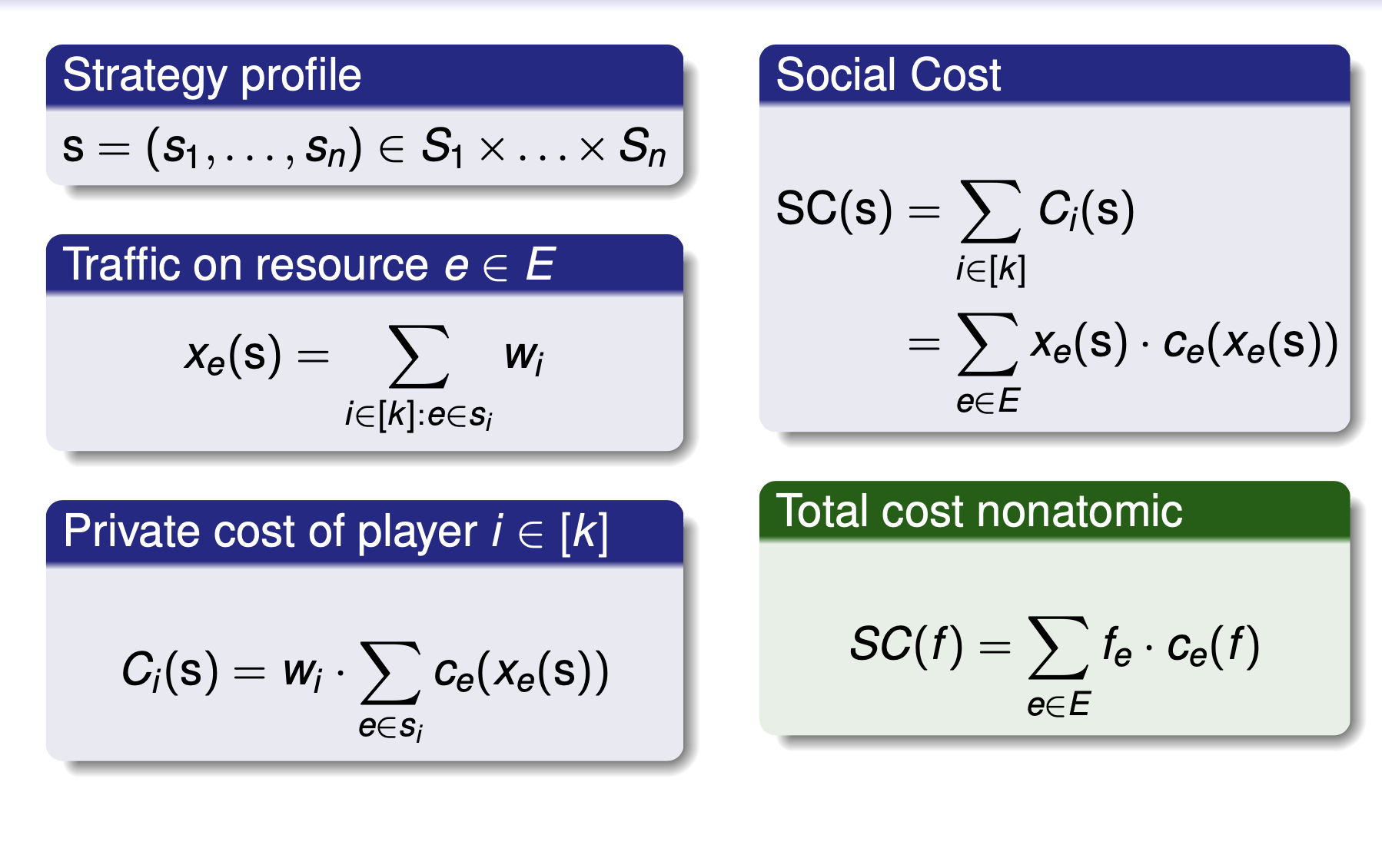
Nash Equilibrium

A strategy profile s is a Nash equilibrium if and only if all players i ∈ [k] are satisfied, that is, Ci(s) ≤ Ci(s−i,si′) for all i ∈ [k] and si′ ∈ Si.

• Remarks
  • For simplicity were strict to pure Nash equilibria.
  • Many result shold also for mixed Nash equilibria.
    • Players randomize over their pure strategies
    • Guaranteed to exist [ NASH, 1951]

Price of Anarchy

Existence of pure NE: positive result

• Theorem 3.6

Every unweighted congestion game possesses a pure Nash equilibrium.

Potential Games and Price of Stability

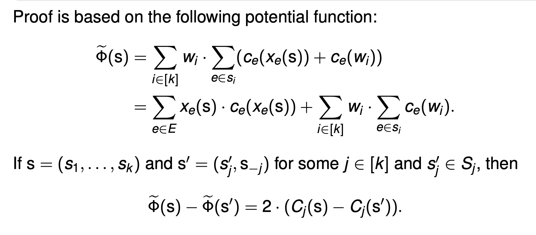
• Potential Games: AllgamesthatadmitapotentialfunctionΦ,s.t.foralloutcomess, all player i, and all alternative strategies si′,

  Ci (si′, s−i ) − Ci (s) = Φ(si′, s−i ) − Φ(s).

• Every congestion game is a potential game.

• For every potential game there exists a congestion game having the same potential function.

• Theorem 3.7

  • There is a weighted network congestion game that does not admit a pure Nash equilibrium.

  

• Theorem 3.8

  • Every weighted congestion game with linear latency functions possesses a pure Nash equilibrium.

  

• Pirce of Anarchy Example:

  

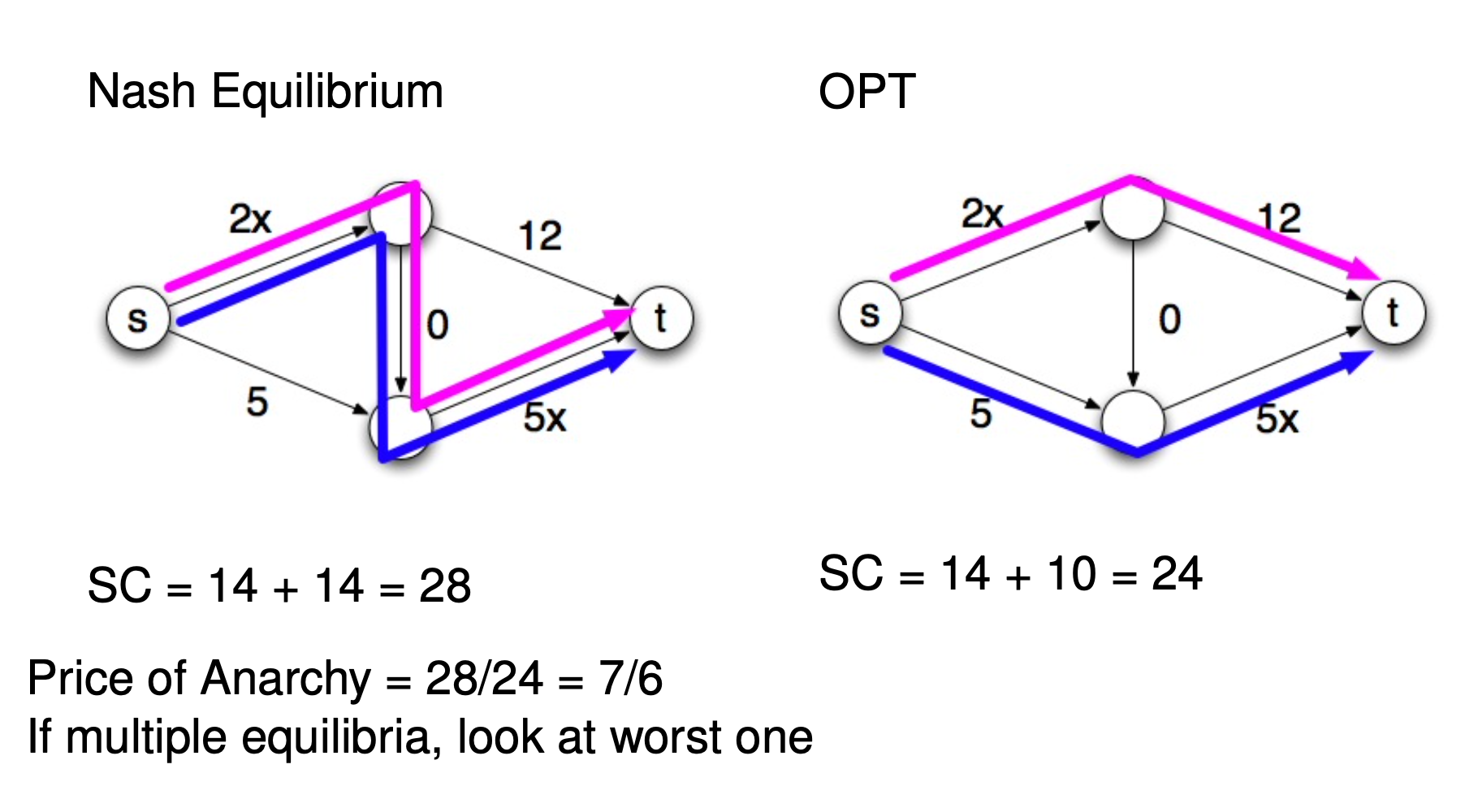
Price of Anarchy: Routing Games

• Analytical simple classes of cost functions ⇒ exact formula for PoA.

  • Linear

  • bounded degree polynomials 有界次多项式

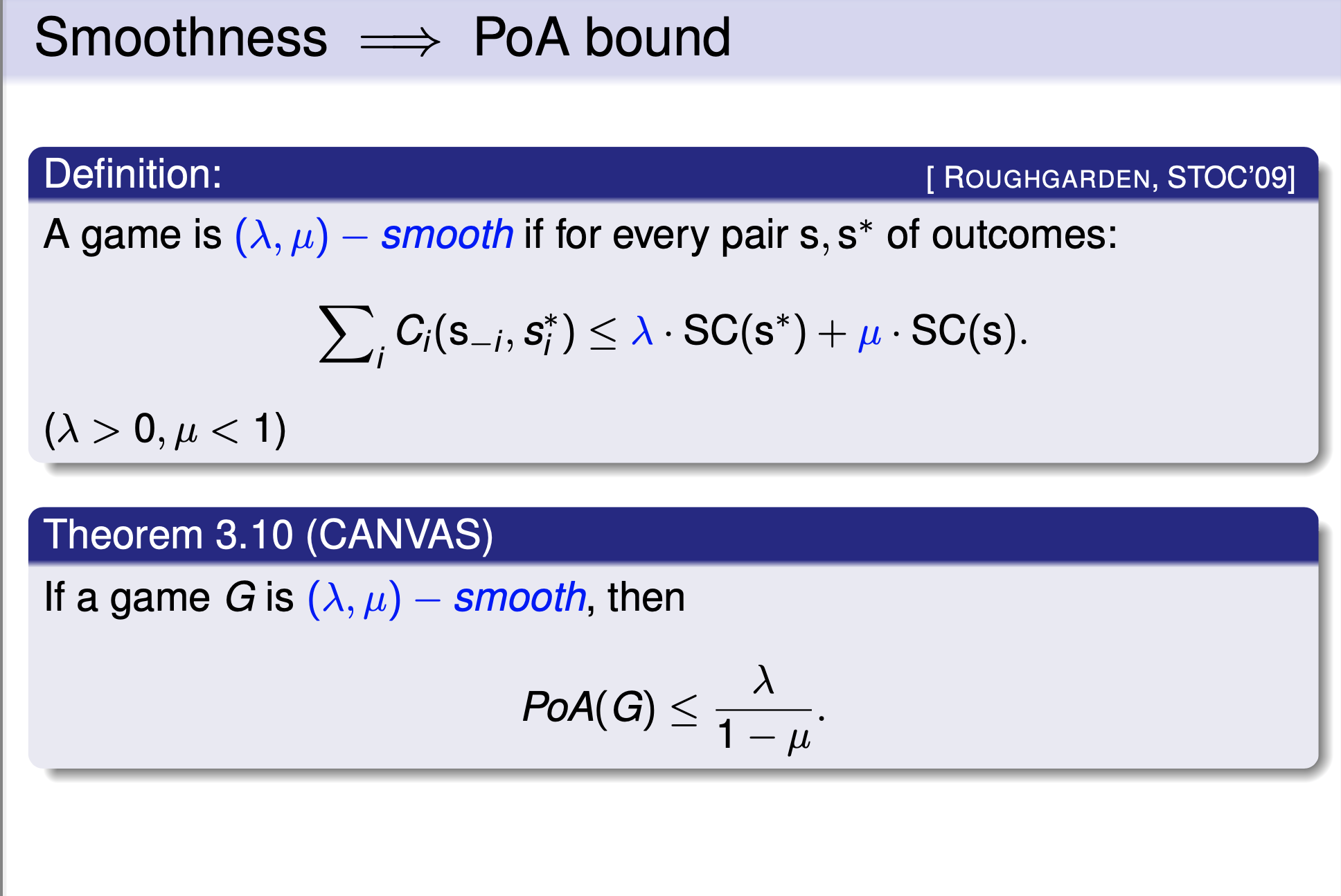
• Theorem 3.9

  • Suppose latency functions are linear with non-negative slope and offset. Then for unweighted games the PoA is exactly 5/2.

    // 假设延迟函数是线性的，具有非负斜率和偏移。对于未加权的游戏，PoA 恰好是 5/2。

• For every set of allowable cost functions ⇒ recipe for computing PoA.

  • non-atomic (Wardrop model)

  • unweighted

Abstract Setup 抽象系统