Derandomisation and Randomised Rounding

Derandomisation

• Sometimes it is possible to “derandomise” a randomised algorithm Arand and obtain a deterministic algorithm Adet.

• The performance of Adet is the same as the expected performance of Arand.

• When successful, we can use randomisation at no extra cost!

(except a polynomial running time overhead).

• Different methods for derandomisation.

  • Can be very complicated (pseudo-random generators).

  • Can be relatively simple (conditional expectations).

• Algorithm: For each variable xi, set xi to 1 with probability 1/2 and to 0 with probability 1/2.

• Algorithm: Set variable xi to 1 or 0 deterministically, and the remaining variables to 1 with probability 1/2 and to 0 with probability 1/2, as before.

• To maximise the expected value W of the algorithm.

• If 𝑊 is the number of clauses satisfied then we have:

  𝔼[𝑊] = 𝔼[𝑊|𝑥 ←1]⋅Pr[𝑥 ←1]+𝔼[𝑊|𝑥 ←0]⋅Pr[𝑥 ←0] = 1/2 (𝔼[𝑊|𝑥 ←1] * +𝔼[𝑊|𝑥 ←0])

• We set x1 to 1 if 𝔼[𝑊|𝑥1 ← 1] ≥ 𝔼[𝑊|𝑥1 ← 0] and to 0 otherwise.

• Generally, if b1 is picked to maximise the conditional expectation, it holds that: 𝔼[𝑊|𝑥 ←𝑏 ]≥𝔼[𝑊]

Applying this to all variables

• Assume that we have set variables x1, …, xi to b1, … bi this way.

• We set xi+1 to 1 if this holds and to 0 otherwise.

𝔼[𝑊|𝑥1 ← 𝑏1,𝑥2 ← 𝑏2,…,𝑥i ← 𝑏i,𝑥i+1 ← 1]≥ 𝔼[𝑊|𝑥1 ← 𝑏1,𝑥2 ← 𝑏2,…,𝑥i ← 𝑏i, 𝑥i+1 ← 0]

• Again, if bi+1 is picked to maximise the conditional expectation, it holds that:

  𝔼[𝑊|𝑥1 ← 𝑏1,𝑥2 ← 𝑏2,…,𝑥i ← 𝑏i,𝑥i+1 ← 𝑏i+1] ≥ 𝔼[𝑊]

In the end

• In the end we have set all variables deterministically (去随机化).

• We have 𝔼[𝑊|𝑥1 ← 𝑏1,𝑥2 ← 𝑏2,…,𝑥i ← 𝑏i,𝑥i+1 ← 𝑏i+1] ≥ 𝔼[𝑊]

• We know that E[W] ≥ 1/2 * OPT

• We have devised a deterministic 2-approximation algorithm.

• Is it polynomial-time? Yes

Computing the expectations

• We have to be able to compute the conditional expectations in polynomial time.

𝔼[𝑊|𝑥1 ← 𝑏1 ,…,𝑥i ←𝑏i]= ∑𝔼[𝑌|𝑥1 ←𝑏1 ,…,𝑥i ←𝑏i]

= ∑ i=1^m Pr[clause𝐶issatisfied|𝑥 ←𝑏 ,…,𝑥 ←𝑏]

• The probability is

  • 1 if the variables already set satisfy the clause.

  • 1-(1/2)k otherwise, where k is the set of unset variables.

Method of conditional expectations

• Derandomisation using conditional expectations.

• Works for a wide variety of applications as long as

  • The variables are set independently.

  • The conditional expectations can be calculated in polynomial time.

Recall: Deterministic Rounding

• For the case of vertex cover we can solve the LP-relaxation in polynomial time, to find an optimal solution.

• The optimal solution is a “fractional” vertex cover, where variables can take values between 0 and 1.

• We round the fractional solution to an integer solution.

  • We pick a variable xi and we set it to 1 or 0.

  • If we set everything to 0, it is not a vertex cover.

  • If we set everything to 1, we “pay” too much.

  • We set variable xi to 1 if xi ≥ 1/2 and to 0 otherwise.

Randomised Rounding

• We formulate the problem as an ILP.

• We write the LP-relaxation.

• We solve the LP-relaxation.

• We round the variables with probabilities that can depend on their values.

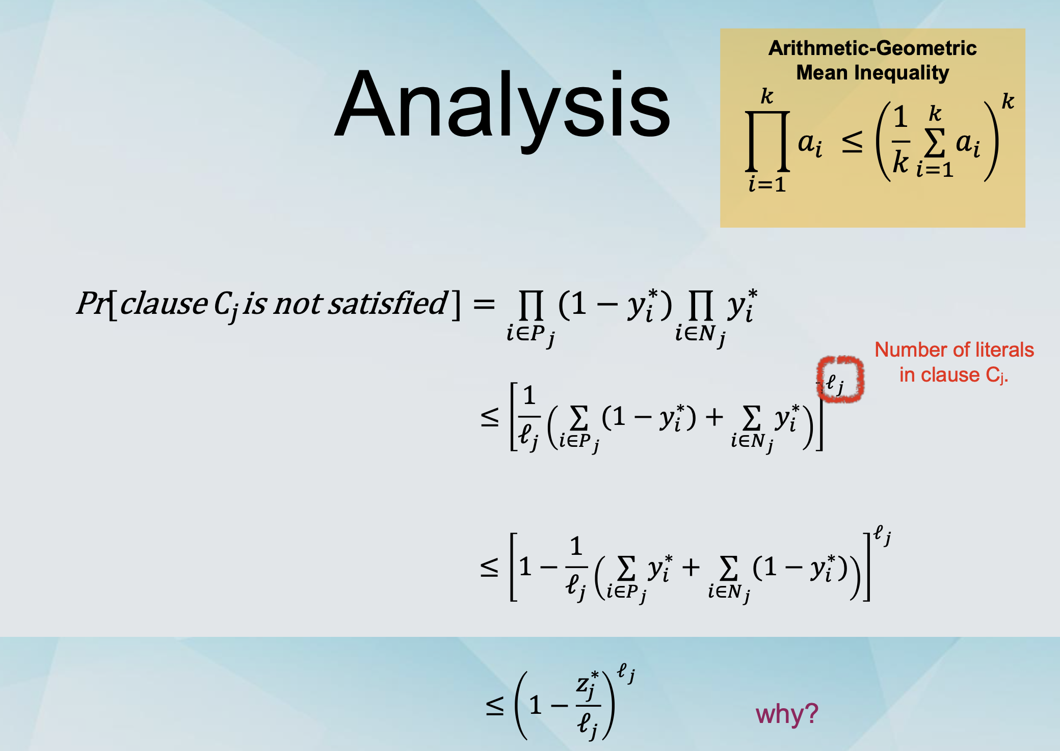
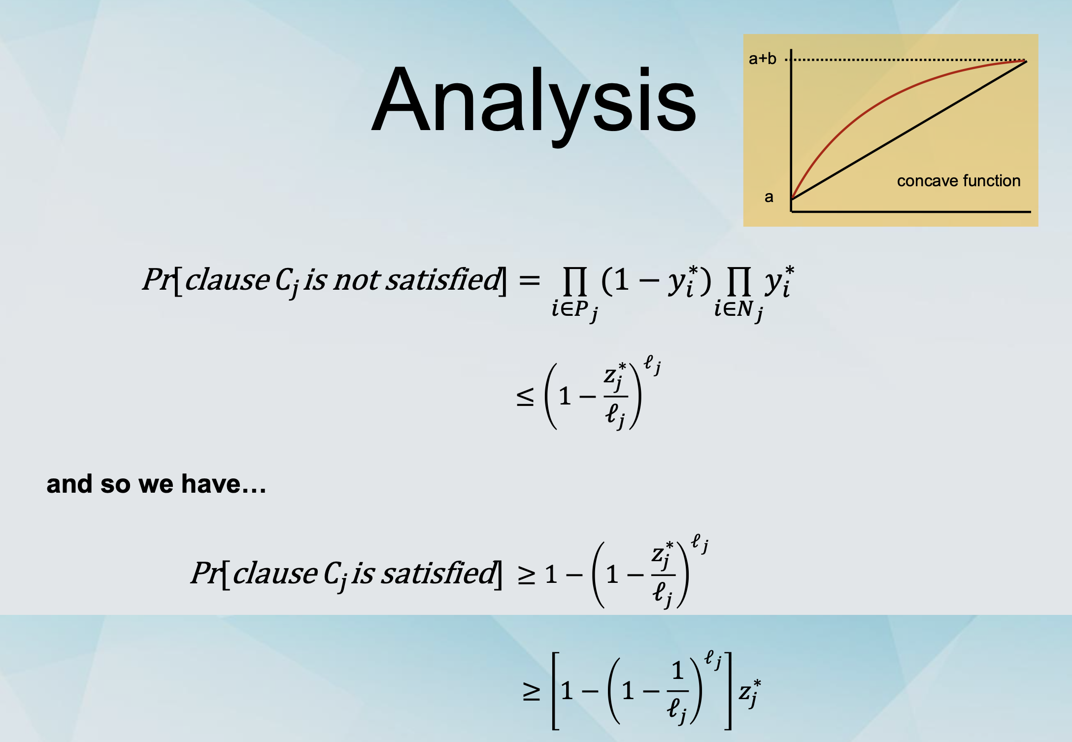
• Let (y*, z*) be a solution to the LP-relaxation.

• Rounding: Set xi to true independently with probability yi*.

  • e.g., if y* = (1/3, 1/4, 5/6, 1/2, …) we will set variables x1, x2, x3, x4, … to true with probabilities 1/3, 1/4, 5/6, 1/2, … respectively.

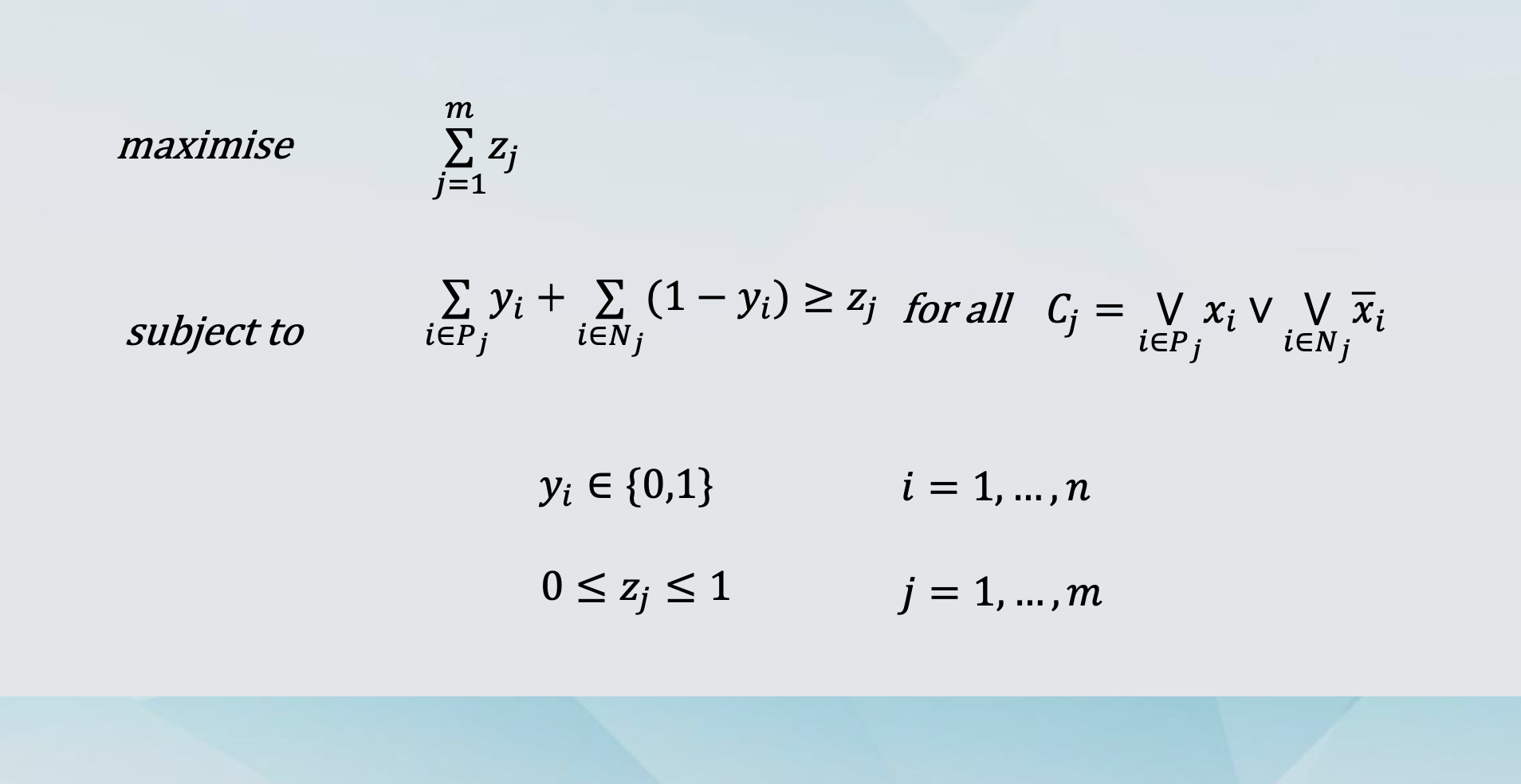
MAX SAT as an ILP

Variables: yi = 1 if xi is true and 0 otherwise.

We denote clause Cj by ⋁ 𝑥𝑖 ∨ ⋁ 𝑥𝑖 𝑖∈𝑃𝑗 𝑖∈𝑁𝑗

Variables: zj = 1 if clause Cj is satisfied and 0 otherwise.

We have the inequality: ∑ 𝑦i + ∑ (1 − 𝑦i ) ≥ 𝑧j

Randomised Rounding for MAX-SAT

• Our randomised algorithm gives an approximation ratio of 1/(1-1/e) ≈ 1.59.

• This is better than 2.

• This is better than 1.618. (why this?)

• Sidenote: 1.618 = φ.

The better of the two

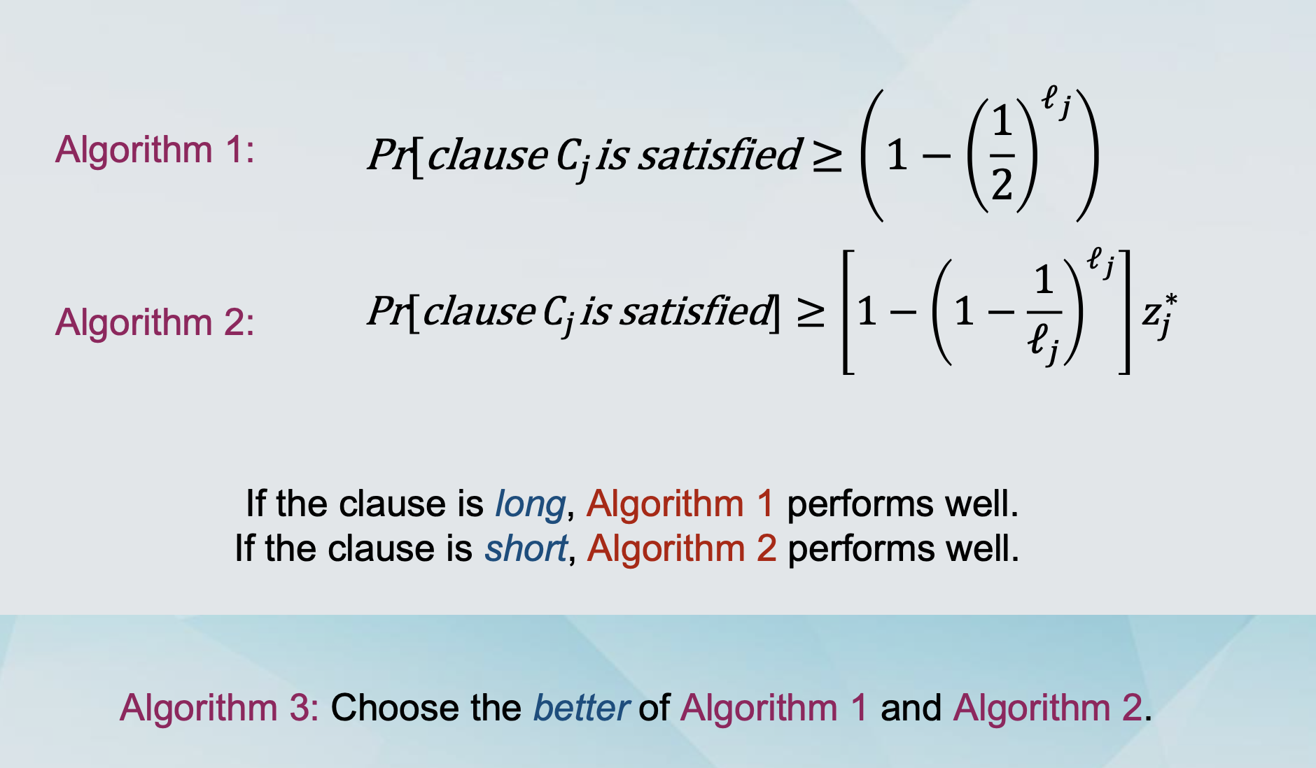
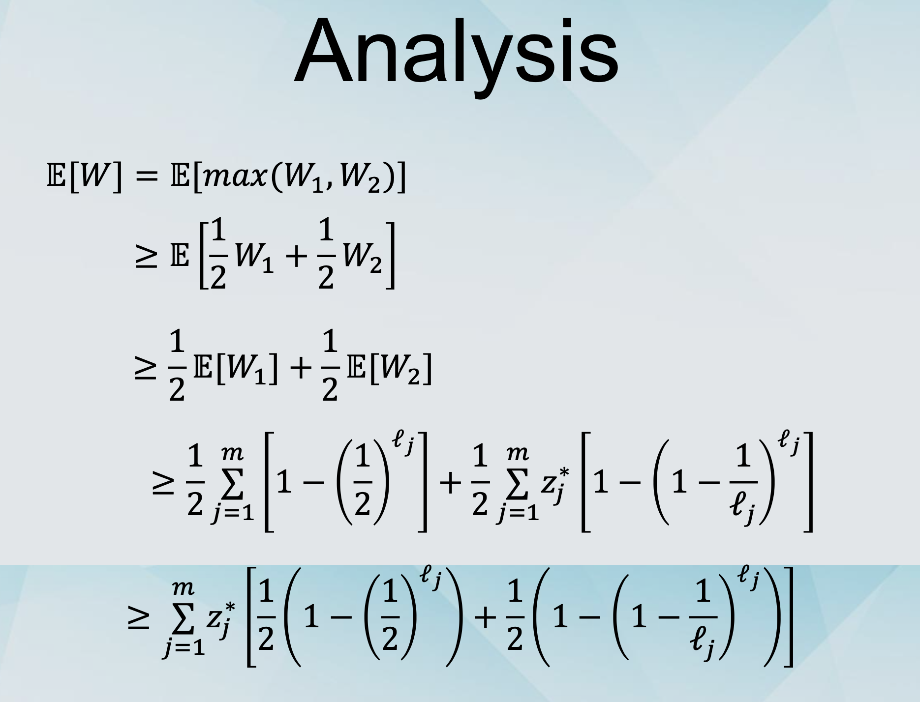
Algorithms for MAX-SAT

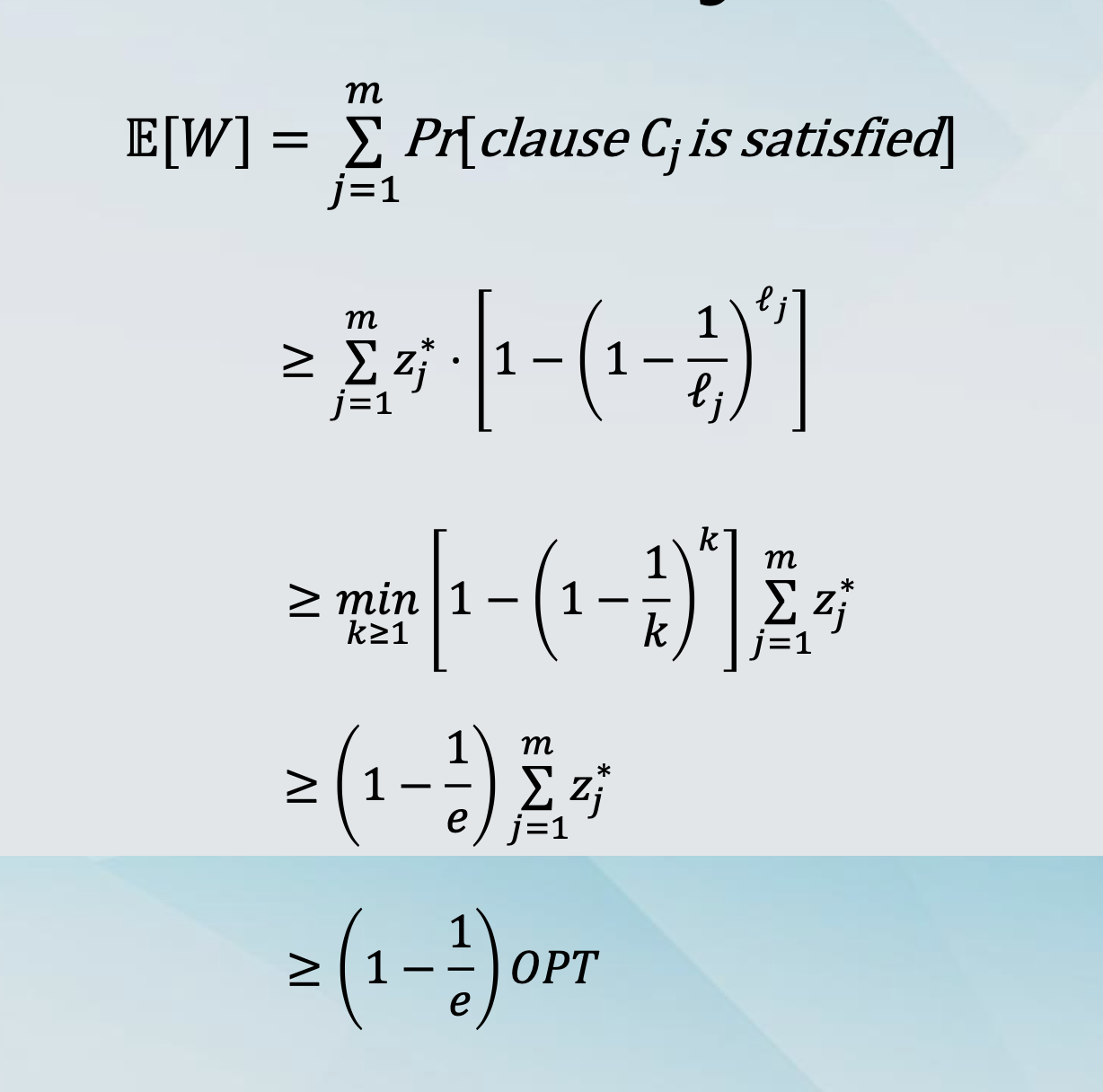
• Our Randomised Rounding algorithm gives an approximation ratio of 1/(1-1/e) ≈ 1.59.

• This is better than 2. (unbiased coin flip for each variable)

• This is better than 1.618. (why this?)

  • Sidenote: 1.618 = φ.

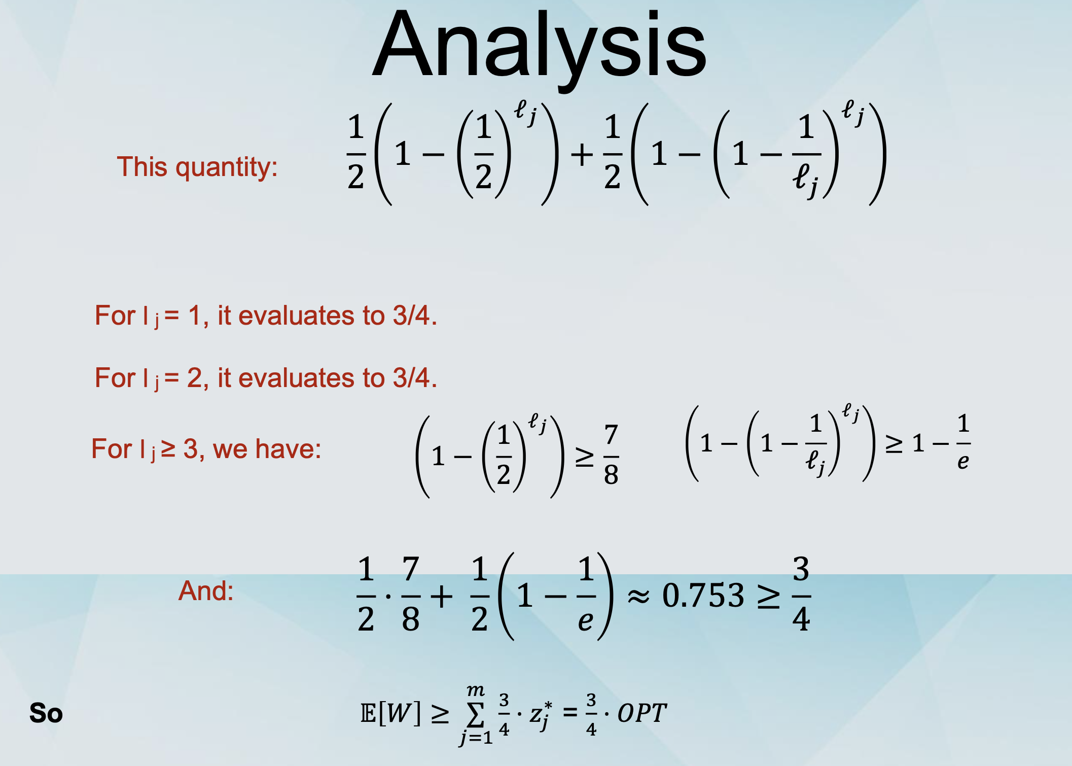
• The “better of the two” algorithm has approximation ratio 4/3 ≈ 1.33.

Back to Randomised Rounding

• Is our RR algorithm the best possible?

• How do we (attempt to) show that?

  • Integrality gap.

Integrality Gap of MAX-SAT

• Consider the formula: (x1 ⌵x2)⌃(┐x1 ⌵x2)⌃(x1 ⌵┐x2)⌃(┐x1 ⌵┐x2)

• The optimal integral solution satisfied 3 clauses.

• The optimal fractional solution sets

  y1= y2 = 1/2 and zj = 1 for all j and satisfies 4 clauses.

• The integrality gap is at least 4/3.

What does this mean?

• We can not hope to design an LP-relaxation and rounding-based algorithm (for this ILP formulation) that outperforms our “better of the two” algorithm.

• Can we design one that matches the 4/3 approximation ratio?

• Yes we can!

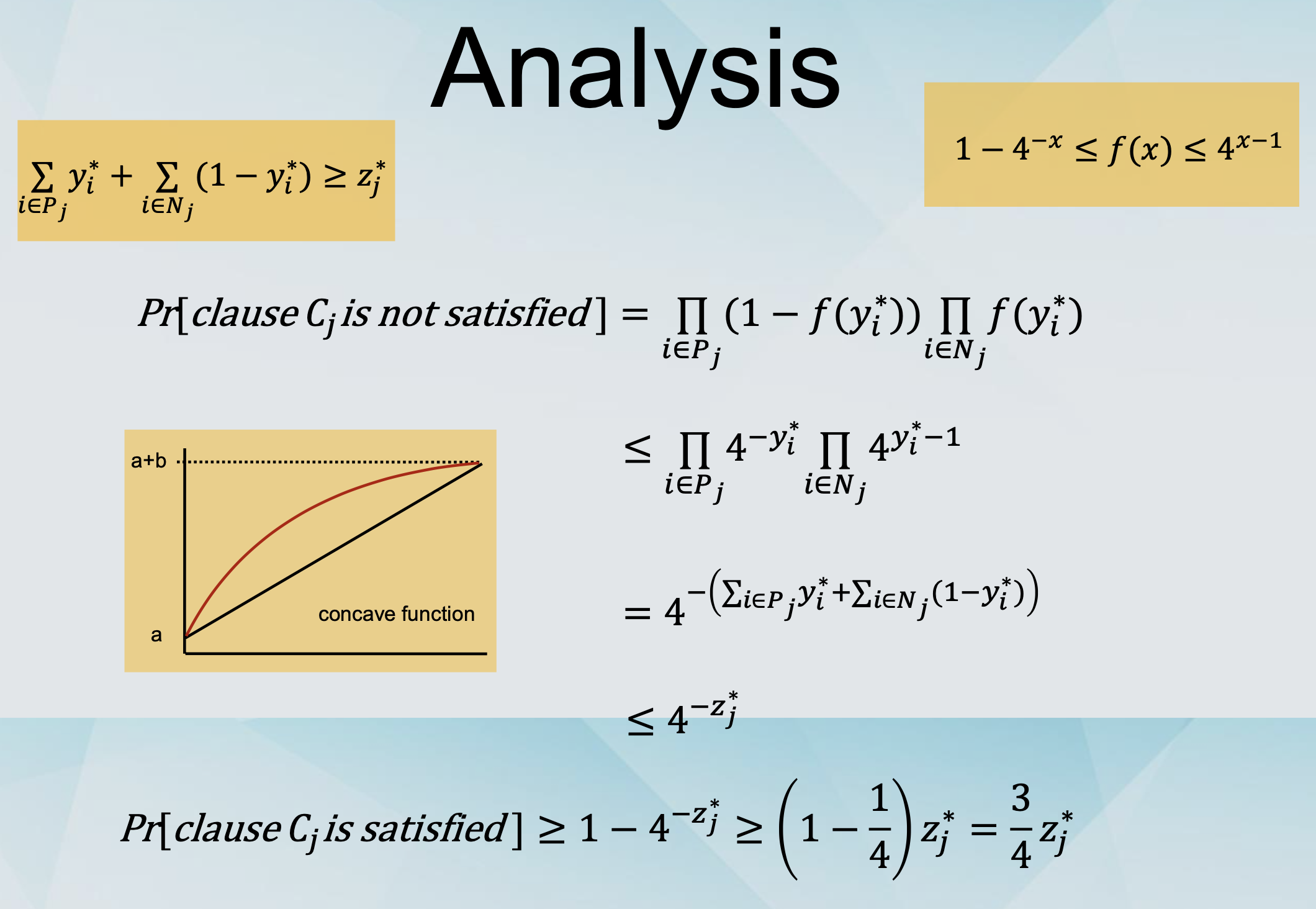
  • Instead of “Set xi to true independently with probability yi*”,

  • We use “Set xi to true independently with probability f(yi*), for some function f.

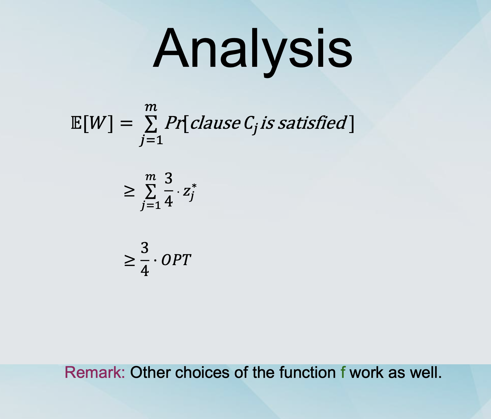
  • Which function f?

    • Any function such that 1 - 4-x ≤ f(x) ≤ 4x-1

Algorithms for MAX-SAT

• Our first RR algorithm gives an approximation ratio of 1/(1-1/e) ≈ 1.59.

• This is better than 2. (fair coin flip for all variables)

• This is better than 1.618. (optimal coin flip for all variables)

• The “better of the two” algorithm has approximation ratio 4/3 ≈ 1.33.

• The more sophisticated RR algorithm has an approximation ratio of 4/3 ≈ 1.33.